[1] 262.0594Promizing Zone Design with rpact
Nestlé rpact Training 2024, Lausanne
May 24, 2024
A Motivating Example from Hsiao, Liu, and Mehta (Biometrical Journal, 2019)
- Efficacy endpoint PFS
- Assumed hazard ratio = 0.67, \(\alpha = 0.025\) and \(\beta = 0.1\) requires 263 events:
- 280 PFS events yields power 91.8 %:
- If 350 patients are enrolled over 28 months with a median PFS time of 8.5 months in the control group, the final analysis is expected to be after an additional follow-up of about 12 months:
getPowerSurvival(alpha = 0.025, hazardRatio = 0.67,
            directionUpper = FALSE,
            maxNumberOfEvents = 280,
            maxNumberOfSubjects = 350,
            median2 = 8.5,
            accrualTime = 28)$analysisTime
[,1]
[1,] 40.52321- 500 PFS events are needed to have 90% power at HR = 0.75 with more patients and a different expected follow-up:
“Milestone-based” investment:
Two-stage approach with interim after 140 events
Enough power for detecting HR = 0.67
If conditional power CP for detecting HR = 0.75 falls in a “promizing zone”, an additional investment would be made that allows the trial to remain open until 420 PFS events were obtained
Conditional power based on assumed minimum clinical relevant effect HR = 0.75
Promizing Zone Design
Number of events for the second stage between 140 and 280
If conditional power for 280 additional events at HR = 0.75 is smaller than \(cp_{min}\), set number of additional events = 140 (non-promising case)
If conditional power for 140 additional events at HR = 0.75 exceeds \(cp_{max}\), set number of additional events = 140, otherwise calculate event number according to \[CP_{HR = 0.75} = cp_{max}\] (promising case)
This defined a promizing zone for HR within the sample size may be modified.
Promizing Zone Design Using rpact
First, define the design
Define the event number calculation function myEventSizeCalculationFunction()
# Define promizing zone event size function
myEventSizeCalculationFunction <- function(..., stage,
                     plannedEvents,
                     conditionalPower,
                     minNumberOfEventsPerStage,
                     maxNumberOfEventsPerStage,
                     conditionalCriticalValue,
                     estimatedTheta) {

  calculateStageEvents <- function(cp) {
      4 * max(0, conditionalCriticalValue + qnorm(cp))^2 /
      log(max(1 + 1e-12, estimatedTheta))^2
  }

  # Calculate events required to reach maximum desired conditional power
  # cp_max (provided as argument conditionalPower)
  stageEventsCPmax <- ceiling(calculateStageEvents(cp = conditionalPower))

  # Calculate events required to reach minimum desired conditional power
  # cp_min (**manually set for this example to 0.8**)
  stageEventsCPmin <- ceiling(calculateStageEvents(cp = 0.8))

  # Define stageEvents
  stageEvents <- min(max(minNumberOfEventsPerStage[stage], stageEventsCPmax),
    maxNumberOfEventsPerStage[stage])

  # Set stageEvents to minimal sample size in case minimum conditional power
  # cannot be reached with available sample size
  if (stageEventsCPmin > maxNumberOfEventsPerStage[stage]) {
    stageEvents <- minNumberOfEventsPerStage[stage]

  }
  # return overall events for second stage
  return(plannedEvents[1] + stageEvents)
}
Run the Simulation
by specifying calcEventsFunction = myEventSizeCalculationFunction and a range of assumed true hazard ratios
simSurvPromZone <- getSimulationSurvival(design = myDesign,
                      hazardRatio = hazardRatioSeq,
                      directionUpper = FALSE,
                      plannedEvents = c(140, 280),
                      median2 = 8.5,
                      minNumberOfEventsPerStage = c(NA, 140),
                      maxNumberOfEventsPerStage = c(NA, 280),
                      thetaH1 = 0.75,
                      conditionalPower = 0.9,
                      accrualTime = 36,
                      calcEventsFunction = myEventSizeCalculationFunction,
                      maxNumberOfIterations = maxNumberOfIterations,
                      longTimeSimulationAllowed = TRUE,
                      maxNumberOfSubjects = 500)
“Usual” Conditional Power Approach
Specify calcEventsFunction = NULL
simSurvCondPower <- getSimulationSurvival(design = myDesign,
hazardRatio = hazardRatioSeq,
directionUpper = FALSE,
plannedEvents = c(140, 280),
median2 = 8.5,
minNumberOfEventsPerStage = c(NA, 140),
maxNumberOfEventsPerStage = c(NA, 280),
thetaH1 = 0.75,
conditionalPower = 0.9,
accrualTime = 36,
calcEventsFunction = NULL,
maxNumberOfIterations = maxNumberOfIterations,
longTimeSimulationAllowed = TRUE,
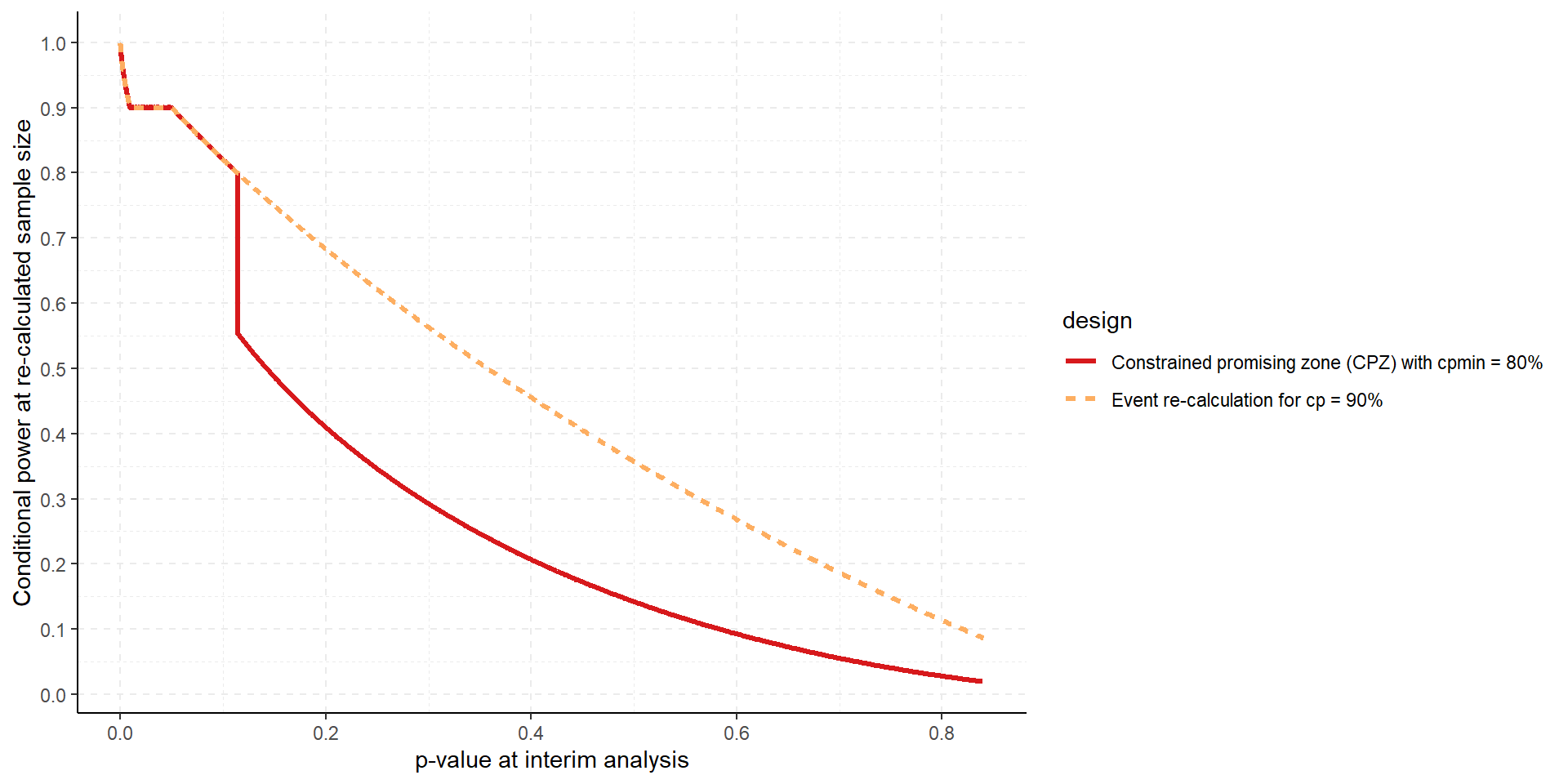
maxNumberOfSubjects = 500) Comparison of Approaches
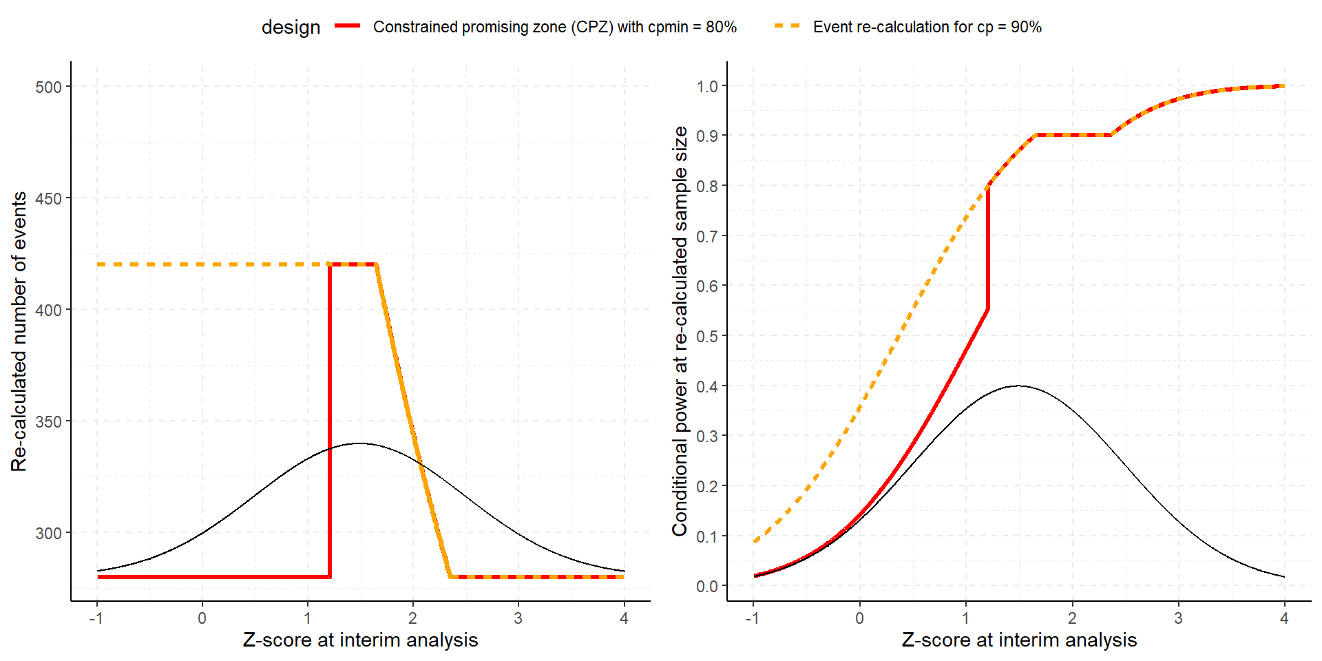
Don’t Increase for, e.g., p = 0.15?
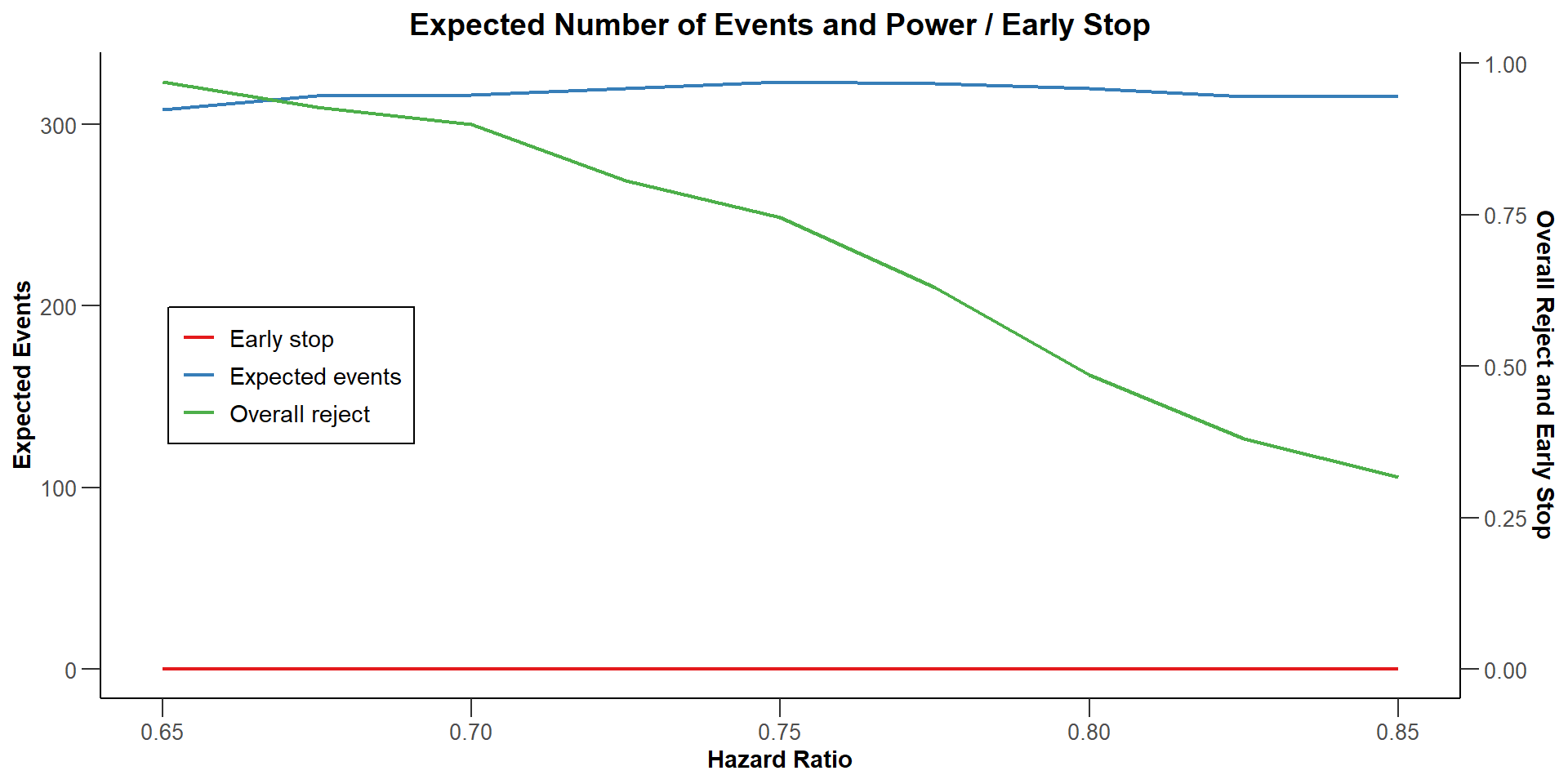

Difference in Power

Difference in Expected Sample Size
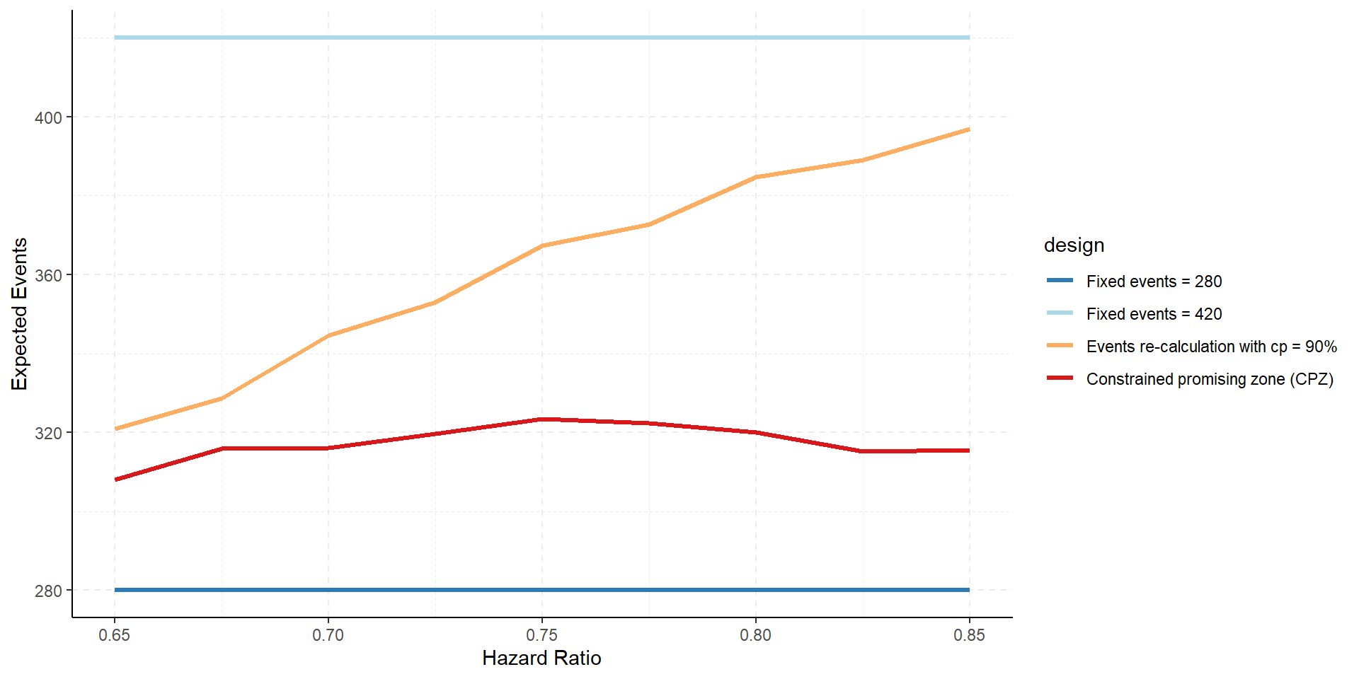
Summary
- Easy implementation in
rpact - Simulation very fast
- Consideration of efficacy or futility stops straightforward
- Trade-off between overall expected sample size and power
- Usage of combination test (or equivalent) theoretically mandatory
- Adaptations based on test statistic only