Using rpact with Raw Data
Nestlé rpact Training 2024, Lausanne
May 24, 2024
Introduction
We show how to use the function getDataset() as an utility function to process adjusted means and estimated standard deviations from raw data, how to convert the raw data into an rpact dataset, and finally how to use this information for the analysis at interim and the final stage. Essentially, this is through the use of the CRAN package emmeans that allows the extraction of least squares means from a specified model, e.g., an ANCOVA model considered here.
What will be illustrated?
- How to import raw data from a SAS file
- How to get the adjusted means and standard deviations from the data
- How to convert the raw data into an dataset
- How to analyze the dataset
Load required R packages
Analysis of raw data – Data import from csv file
Artificial dataset that was randomly generated with simulated normal data.
The dataset has six variables:
- Subject id
- Stage number
- Group name
- An example
outcomein that we are interested in - The first covariate
gender - The second covariate
covariate
data <- read.csv(file = "../files/data_two_arm_adjusted_means.csv")
data <- data[, !(colnames(data) %in% c("visit", "seed"))]
data1 <- data[data$stage == 1, ]
data2 <- data[data$stage == 2, ]
data3 <- data[data$stage == 3, ]
head(data1)
subject stage group outcome gender covariate
1 1101 1 Treatment group 60.91533 m 41.74395
2 1102 1 Treatment group 57.65198 f 43.94315
3 1103 1 Treatment group 118.36755 f 38.82385
4 1104 1 Treatment group 118.25124 m 36.79198
5 1105 1 Treatment group 174.35321 f 42.92030
6 1106 1 Treatment group 113.80682 f 36.30031Analysis of raw data – Descriptive Statistics
s1 <-aggregate(x = data$outcome, by = list(data$group,
    data$stage), FUN = mean, na.rm = TRUE)
s2 <-aggregate(x = data$outcome, by = list(data$group,
    data$stage), FUN = sd, na.rm = TRUE)
s3 <-aggregate(x = data$outcome, by = list(data$group,
    data$stage), FUN = length)
tab <- data.frame(stage = s1$Group.2,
                    arm = s1$Group.1,
                    n = s3$x,
                    mean = s1$x,
                    std = s2$x) |>
    print()
stage arm n mean std
1 1 Control group 87 91.66591 49.13310
2 1 Treatment group 87 110.88731 45.65258
3 2 Control group 87 101.83443 41.97826
4 2 Treatment group 87 114.06969 49.06744
5 3 Control group 87 103.31525 37.87368
6 3 Treatment group 87 112.17591 39.91061The mean of outcome is larger in the treatment group as in the control group.
Check whether group is a character vector or factor:
Convert group to a factor (so that the order can be changed later):
\(\hspace{1.5cm}\)
Since its first release, R has by default converted character strings to factors when creating data frames directly with data.frame() or as the result of using read.table() variants (e.g., read.csv()) to read in tabular data, i.e., stringsAsFactors = TRUE by default.
With the release of R 4.0.0 the default was changed to stringsAsFactors = FALSE!
Explore covariates
Frequency of gender levels per group:
The frequency of gender has a good balance, overall and per group.
Interim analyses
First look: analysis at stage 1
For illustration we create a group sequential design with default parameters:
Then we create a linear model with dependent variable y = outcome, independent variable group, and covariates covariate and gender, i.e., the model formula is outcome ~ group + covariate + gender:
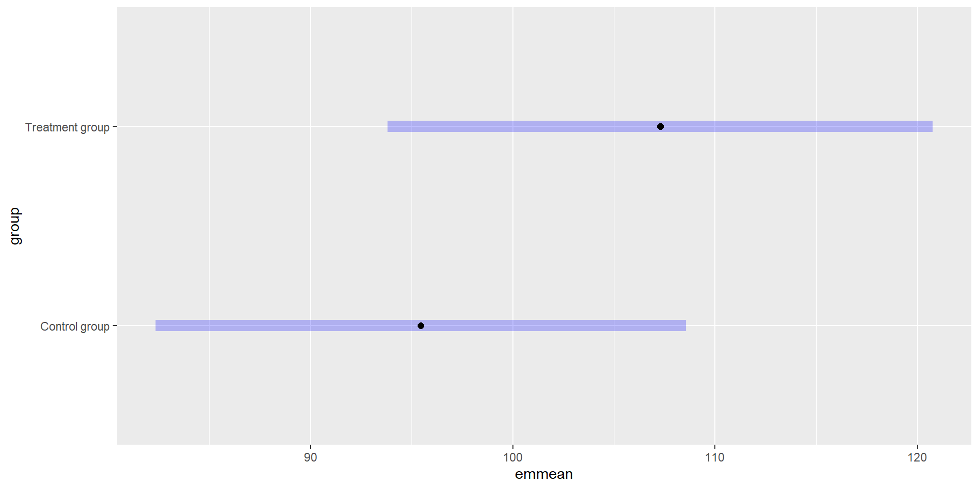
Here we are not interested in the model output but we need it to compute the estimated marginal means (EMMs; least-squares means) for the factor group in the model:
 group           emmean   SE  df lower.CL upper.CL
 Control group     95.4 6.64 167     82.3      109
 Treatment group  107.3 6.82 167     93.8      121

Results are averaged over the levels of: gender
Confidence level used: 0.95
Note that the estimated standard deviation is also included in the object.
The rpact function getDataset() directly accepts the result objects of emmeans(). To create the dataset for the first interim analysis we only have to put the object emResult1 as exclusive argument to the function getDataset():
Check the getDataset result
The order of the group levels is important to get the correct analysis results. Therefore we do some check before we continue.
rpact expects the following group level order:
- 1 = Treatment group
- 2 = Control group
Carefully check and define the order of the group levels. Depending on the group names it is important to guarantee that the order is defined as expected from rpact (see above).
For correct modelling, the control group should be the reference level and is therefore set to position 1:
Alternative command to reorder the group levels:
If the treatment group shall be the reference level you can later add the argument directionUpper = FALSE to getAnalysisResult().
After modifying the order double check that the dataset is still correct. We do that by creating the unadjusted dataset using a simple model without covariates:
datasetCheck1 <- getDataset(
    emmeans(lm(outcome ~ group, data = data1), "group"))
tapply(datasetCheck1$means, datasetCheck1$groups, mean, na.rm = TRUE)
1 2
110.88731 91.66591 Control group Treatment group
91.66591 110.88731 The control group has a mean of 91.7 in the raw data and in the dataset, where 2 = control.
Recalculate the estimated marginal means for the complete model:
The estimated marginal means and corresponding confidence intervals within the strata of the factors of the model can be obtained as follows:
 group           covariate gender emmean   SE  df lower.CL upper.CL
 Control group        45.3 f       100.7 7.45 167     86.0      115
 Treatment group      45.3 f       112.6 7.94 167     96.9      128
 Control group        45.3 m        90.2 7.68 167     75.0      105
 Treatment group      45.3 m       102.0 7.50 167     87.2      117

Confidence level used: 0.95
Analysis results of stage 1
As from above, let dataset1 be the dataset for the complete model:
Analysis results of stage 1
Analysis results for a continuous endpoint
Sequential analysis with 3 looks (group sequential design). The results were calculated using a two-sample t-test (one-sided, alpha = 0.025), equal variances option. H0: mu(1) - mu(2) = 0 against H1: mu(1) - mu(2) > 0.
| Stage | 1 | 2 | 3 |
|---|---|---|---|
| Planned information rate | 0.333 | 0.667 | 1 |
| Efficacy boundary (z-value scale) | 3.471 | 2.454 | 2.004 |
| Cumulative alpha spent | 0.0003 | 0.0072 | 0.0250 |
| Stage level | 0.0003 | 0.0071 | 0.0225 |
| Cumulative effect size | 11.836 | ||
| Cumulative (pooled) standard deviation | 62.192 | ||
| Overall test statistic | 1.244 | ||
| Overall p-value | 0.1076 | ||
| Test action | continue | ||
| Conditional rejection probability | 0.0621 | ||
| 95% repeated confidence interval | [-21.835; 45.506] | ||
| Repeated p-value | 0.3127 |
The test decision at stage 1 is to not reject the null hypothesis and to continue the trial.
If the treatment group shall be the reference level you may add directionUpper = FALSE (default is TRUE):
data1b <- data1
data1b$group <- relevel(data1b$group, ref = "Treatment group")
dataset1b <- getDataset(emmeans(lm(
    outcome ~ group + covariate + gender,
    data = data1b), "group"))
analysisResults1b <- getAnalysisResults(
    design = design,
    dataInput = dataset1b, directionUpper = FALSE
)
summary(analysisResults1b)
Analysis results for a continuous endpoint
Sequential analysis with 3 looks (group sequential design). The results were calculated using a two-sample t-test (one-sided, alpha = 0.025), equal variances option. H0: mu(1) - mu(2) = 0 against H1: mu(1) - mu(2) < 0.
| Stage | 1 | 2 | 3 |
|---|---|---|---|
| Planned information rate | 0.333 | 0.667 | 1 |
| Efficacy boundary (z-value scale) | 3.471 | 2.454 | 2.004 |
| Cumulative alpha spent | 0.0003 | 0.0072 | 0.0250 |
| Stage level | 0.0003 | 0.0071 | 0.0225 |
| Cumulative effect size | -11.836 | ||
| Cumulative (pooled) standard deviation | 62.192 | ||
| Overall test statistic | -1.244 | ||
| Overall p-value | 0.1076 | ||
| Test action | continue | ||
| Conditional rejection probability | 0.0621 | ||
| 95% repeated confidence interval | [-45.506; 21.835] | ||
| Repeated p-value | 0.3127 |
Repeated confidence interval: values turn around from [-21.8; 45.5] to [-45.5; 21.8].
Second look: analysis at stage 2
Similar to stage 1, we create a linear model with dependent variable y = outcome, independent variable group, and covariates covariate and gender:
Then we calculate the estimated marginal means of this linear model:
To create the dataset for the second interim analysis we only have to put the objects emResult1 and emResult2 as exclusive comma-separated arguments to the function getDataset():
Dataset of means
The dataset contains the sample sizes, means, and standard deviations of one treatment and one control group. The total number of looks is two; stage-wise and cumulative data are included.
| Stage | 1 | 1 | 2 | 2 |
|---|---|---|---|---|
| Group | 1 | 2 | 1 | 2 |
| Stage-wise sample size | 84 | 87 | 79 | 82 |
| Cumulative sample size | 84 | 87 | 163 | 169 |
| Stage-wise mean | 107.284 | 95.448 | 110.150 | 105.487 |
| Cumulative mean | 107.284 | 95.448 | 108.673 | 100.319 |
| Stage-wise standard deviation | 62.477 | 61.916 | 62.075 | 61.662 |
| Cumulative standard deviation | 62.477 | 61.916 | 62.107 | 61.814 |
Display the analysis results for stage 2:
Analysis results for a continuous endpoint
Sequential analysis with 3 looks (group sequential design). The results were calculated using a two-sample t-test (one-sided, alpha = 0.025), equal variances option. H0: mu(1) - mu(2) = 0 against H1: mu(1) - mu(2) > 0.
| Stage | 1 | 2 | 3 |
|---|---|---|---|
| Planned information rate | 0.333 | 0.667 | 1 |
| Efficacy boundary (z-value scale) | 3.471 | 2.454 | 2.004 |
| Cumulative alpha spent | 0.0003 | 0.0072 | 0.0250 |
| Stage level | 0.0003 | 0.0071 | 0.0225 |
| Cumulative effect size | 11.836 | 8.354 | |
| Cumulative (pooled) standard deviation | 62.192 | 61.958 | |
| Overall test statistic | 1.244 | 1.228 | |
| Overall p-value | 0.1076 | 0.1101 | |
| Test action | continue | continue | |
| Conditional rejection probability | 0.0621 | 0.0412 | |
| 95% repeated confidence interval | [-21.835; 45.506] | [-8.430 ; 25.138] | |
| Repeated p-value | 0.3127 | 0.2002 |
The test decision at stage 2 is to not reject the null hypothesis and to continue the trial.
Last look: analysis at stage 3
After collection of the additional trial data planned for stage 3, we can read the raw data, e.g., from a local csv file:
data3 <- data[data$stage == 3, ]
data3$group <- as.factor(data3$group)
data3$group <- relevel(data3$group, ref = "Control group")
head(data3)
subject stage group outcome gender covariate
349 3101 3 Treatment group NA f 37.05855
350 3102 3 Treatment group 132.68682 m 35.38209
351 3103 3 Treatment group 116.46593 m 40.54073
352 3104 3 Treatment group 66.91700 f 40.46552
353 3105 3 Treatment group 47.36712 f 30.74220
354 3106 3 Treatment group 58.37924 f 37.44284[1] 174 6Similar to stages 1 and 2, we create a linear model with dependent variable y = outcome, independent variabe group, and covariates covariate and gender:
Calculate the estimated marginal means of this linear model:
To create the dataset for the third interim analysis we only have to put the objects emResult1, emResult2, and emResult3 as exclusive comma-separated arguments to the function getDataset():
Dataset of means
The dataset contains the sample sizes, means, and standard deviations of one treatment and one control group. The total number of looks is three; stage-wise and cumulative data are included.
| Stage | 1 | 1 | 2 | 2 | 3 | 3 |
|---|---|---|---|---|---|---|
| Group | 1 | 2 | 1 | 2 | 1 | 2 |
| Stage-wise sample size | 84 | 87 | 79 | 82 | 81 | 84 |
| Cumulative sample size | 84 | 87 | 163 | 169 | 244 | 253 |
| Stage-wise mean | 107.284 | 95.448 | 110.150 | 105.487 | 113.769 | 101.753 |
| Cumulative mean | 107.284 | 95.448 | 108.673 | 100.319 | 110.365 | 100.795 |
| Stage-wise standard deviation | 62.477 | 61.916 | 62.075 | 61.662 | 53.135 | 52.656 |
| Cumulative standard deviation | 62.477 | 61.916 | 62.107 | 61.814 | 59.218 | 58.830 |
As final step of stage 3 we create and display the analysis results:
Analysis results for a continuous endpoint
Sequential analysis with 3 looks (group sequential design). The results were calculated using a two-sample t-test (one-sided, alpha = 0.025), equal variances option. H0: mu(1) - mu(2) = 0 against H1: mu(1) - mu(2) > 0.
| Stage | 1 | 2 | 3 |
|---|---|---|---|
| Planned information rate | 0.333 | 0.667 | 1 |
| Efficacy boundary (z-value scale) | 3.471 | 2.454 | 2.004 |
| Cumulative alpha spent | 0.0003 | 0.0072 | 0.0250 |
| Stage level | 0.0003 | 0.0071 | 0.0225 |
| Cumulative effect size | 11.836 | 8.354 | 9.570 |
| Cumulative (pooled) standard deviation | 62.192 | 61.958 | 59.021 |
| Overall test statistic | 1.244 | 1.228 | 1.807 |
| Overall p-value | 0.1076 | 0.1101 | 0.0357 |
| Test action | continue | continue | accept |
| Conditional rejection probability | 0.0621 | 0.0412 | |
| 95% repeated confidence interval | [-21.835; 45.506] | [-8.430 ; 25.138] | [-1.070 ; 20.210] |
| Repeated p-value | 0.3127 | 0.2002 | 0.0404 |
| Final p-value | 0.0374 | ||
| Final confidence interval | [-0.949; 19.884] | ||
| Median unbiased estimate | 9.483 |
The test decision at stage 3 is reject the null hypothesis.
Multi-stage raw data import
Let us assume that the data of the different stages are not stored in different data files but in one dataset where a stage column acts as an identifier for the data of the different stages.
Question: what is an efficient way to put the data to getDataset()?
Solution
First, to enable the later usage of sapply, we write a short function that returns the emmeans of a linear model result that uses only the data at the specified stage.
The arguments of the function are
stageAn integer specifying the stage number.fThe function which shall produce the linear model result, e.g.,stats::lm.formulaThe model formula.dataThe data.frame containing the multi-stage raw data (must contain the columnstage).specsThe specs argument of theemmeans()function (used to specify the name of the group column).
Read the data of all stages:
Then we use the function unique to identify the available stages in the data.frame:
as.integer ensures that the stages will be valid also if data$stage is a factor.
Now we can create the rpact datasets for different model formulas in one step.
Example 1: Simple model without any covariates
Example 1: Simple model without any covariates
Dataset of means
The dataset contains the sample sizes, means, and standard deviations of one treatment and one control group. The total number of looks is three; stage-wise and cumulative data are included.
| Stage | 1 | 1 | 2 | 2 | 3 | 3 |
|---|---|---|---|---|---|---|
| Group | 1 | 2 | 1 | 2 | 1 | 2 |
| Stage-wise sample size | 84 | 87 | 79 | 82 | 81 | 84 |
| Cumulative sample size | 84 | 87 | 163 | 169 | 244 | 253 |
| Stage-wise mean | 110.887 | 91.666 | 114.070 | 101.834 | 112.176 | 103.315 |
| Cumulative mean | 110.887 | 91.666 | 112.430 | 96.600 | 112.345 | 98.829 |
| Stage-wise standard deviation | 48.078 | 48.078 | 46.171 | 46.171 | 39.386 | 39.386 |
| Cumulative standard deviation | 48.078 | 48.078 | 47.045 | 47.298 | 44.567 | 44.859 |
Example 2: Linear model with covariates
Example 2: Linear model with covariates
Dataset of means
The dataset contains the sample sizes, means, and standard deviations of one treatment and one control group. The total number of looks is three; stage-wise and cumulative data are included.
| Stage | 1 | 1 | 2 | 2 | 3 | 3 |
|---|---|---|---|---|---|---|
| Group | 1 | 2 | 1 | 2 | 1 | 2 |
| Stage-wise sample size | 84 | 87 | 79 | 82 | 81 | 84 |
| Cumulative sample size | 84 | 87 | 163 | 169 | 244 | 253 |
| Stage-wise mean | 107.284 | 95.448 | 110.150 | 105.487 | 113.769 | 101.753 |
| Cumulative mean | 107.284 | 95.448 | 108.673 | 100.319 | 110.365 | 100.795 |
| Stage-wise standard deviation | 63.292 | 62.723 | 62.854 | 62.437 | 53.813 | 53.328 |
| Cumulative standard deviation | 63.292 | 62.723 | 62.902 | 62.601 | 59.974 | 59.579 |
Note that the simple model outcome ~ group in this example results in an analysis result that rejects the null hypothesis already at stage 2 because covariate has an effect on the outcome.
Analysis results for a continuous endpoint
Sequential analysis with 3 looks (group sequential design). The results were calculated using a two-sample t-test (one-sided, alpha = 0.025), equal variances option. H0: mu(1) - mu(2) = 0 against H1: mu(1) - mu(2) > 0.
| Stage | 1 | 2 | 3 |
|---|---|---|---|
| Planned information rate | 0.333 | 0.667 | 1 |
| Efficacy boundary (z-value scale) | 3.471 | 2.454 | 2.004 |
| Cumulative alpha spent | 0.0003 | 0.0072 | 0.0250 |
| Stage level | 0.0003 | 0.0071 | 0.0225 |
| Cumulative effect size | 19.221 | 15.830 | 13.516 |
| Cumulative (pooled) standard deviation | 48.078 | 47.174 | 44.716 |
| Overall test statistic | 2.614 | 3.057 | 3.369 |
| Overall p-value | 0.0049 | 0.0012 | 0.0004 |
| Test action | continue | reject and stop | reject |
| Conditional rejection probability | 0.3238 | 0.7934 | |
| 95% repeated confidence interval | [-6.808; 45.251] | [3.051 ; 28.609] | [5.455 ; 21.577] |
| Repeated p-value | 0.0798 | 0.0071 | 0.0004 |
| Final p-value | 0.0014 | ||
| Final confidence interval | [5.438; 25.824] | ||
| Median unbiased estimate | 15.652 |
Conclusions
getDatasetsupportsemmeansresult objects since rpact version 3.1.1- Easy to use: just add one
emmeansresult object per stage as argument ofgetDataset - rpact will support all models that are supported by
emmeans, e.g., complex longitudinal models with random intercept and random slope (not yet supported) - Multi-arm analysis is also supported (carefully define order of treatments and control!)