Delayed Response Designs

Nestlé rpact Training 2024, Lausanne

Gernot Wassmer and Friedrich Pahlke

May 24, 2024

Methodology of Delayed Response Designs

• In rpact version 3.3, the delayed response group sequential methodology from Hampson & Jennison (2013) is implemented. Further work, e.g., by Whitehead (1992), Faldum & Hommel (2007), Schüürhuis (2022)
• Main task was to write a function returning the decision critical values according to the calculation rules in Hampson & Jennison (2013)
• Functions characterizing a delayed response group sequential test given certain input parameters in terms of power, maximum sample size and expected sample size have been written
• These functions were integrated in getDesignGroupSequential(), getDesignCharacteristics(), and the corresponding getSampleSizexxx() and getPowerxxx() functions
• Other approaches can conveniently be handled with the newly published function getGroupSequentialProbabilities().

Methodology of Delayed Response Designs

Consider function getGroupSequentialProbabilities() which provides precentiles within a group sequential design (Armitage & McPherson algorithm):

Example Type I error rate when using the unadjusted critical value in a two-sided design

kMax <- 4
alpha <- 0.05
decisionMatrix <- matrix(c(rep(-qnorm(1-alpha/2), kMax),
                    rep(qnorm(1-alpha/2), kMax)),
                    byrow = TRUE, ncol = kMax)
probs <- getGroupSequentialProbabilities(
                    decisionMatrix = decisionMatrix,
                    informationRates = (1 : kMax)/kMax)
probs

      [,1]      [,2]       [,3]        [,4]
[1,] 0.025 0.0165589 0.01206929 0.009456319
[2,] 0.975 0.9334411 0.90481291 0.883287306
[3,] 1.000 0.9500000 0.91688220 0.892743625

sum(probs[3,] - probs[2,] + probs[1,])

[1] 0.126169

Methodology of Delayed Response Designs

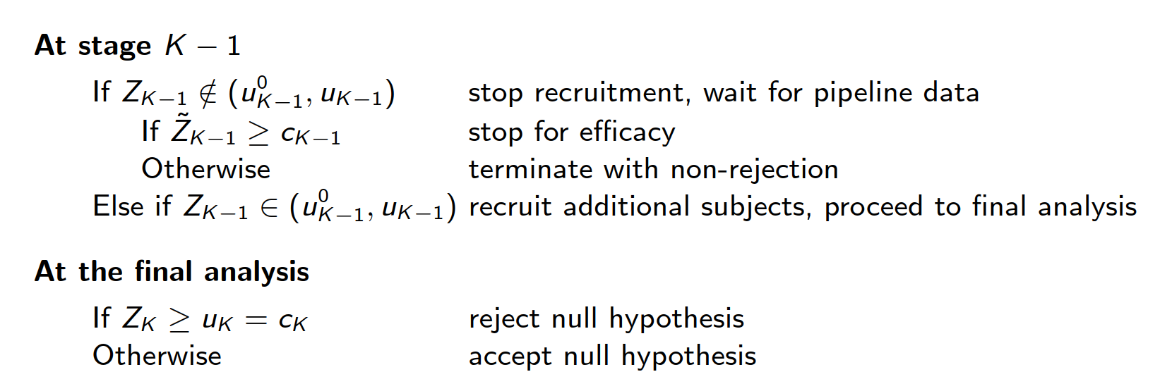
Given boundary sets \(\{u^0_1,\dots,u^0_{K-1}\}\), \(\{u_1,\dots,u_K\}\) and \(\{c_1,\dots,c_K\}\), a \(K\)-stage delayed response group sequential design has the following structure:

• According to Hampson & Jennison (2013), the boundaries \(\{c_1, \dots, c_K\}\) with \(c_K = u_K\) are chosen such that “reversal probabilities” are balanced. More precisely, \(c_1,\ldots,c_{K - 1}\) are chosen as the (unique) solution of:

\[ \begin{split} &P_{H_0}(Z_1 \in (u^0_1, u_1), \dots, Z_{k-1} \in (u^0_{k-1}, u_{k-1}), Z_k \geq u_k, \tilde{Z}_k \leq c_k) \\ &= P_{H_0}(Z_1 \in (u^0_1, u_1), \dots, Z_{k-1} \in (u^0_{k-1}, u_{k-1}), Z_k \leq u^0_k, \tilde{Z}_k \geq c_k). \end{split} \] This ensures Type I error rate control

Methodology of Delayed Response Designs

• Power calculation through

\[ \begin{split} P_{\delta}(&Z_1 \notin (u^0_1, u_1), \tilde{Z}_1 > c_1) \\ &+ \sum_{k=2}^{K-1} P_{\delta}(Z_1 \in (u^0_1, u_1), \dots , Z_{k-1} \in (u^0_{k-1}, u_{k-1}), Z_k \notin (u^0_k, u_k), \tilde{Z}_k \geq c_k) \\ &+ P_{\delta}(Z_1 \in (u^0_1, u_1), \dots , Z_{K-1} \in (u^0_{K-1}, u_{K-1}), Z_K \geq c_K)\,. \end{split} \]

• Maximum sample size, inflation factor, and ASN is calculated for arbitrary \(\delta\), thus test characteristics are easily derived.

Example Decision Critical Values

Use delayedInformation: Delay of information for delayed response designs. Can be a numeric value or a numeric vector of length kMax - 1

gsdWithDelay <- getDesignGroupSequential(
    kMax = 3,
    alpha = 0.025,
    beta = 0.2,
    typeOfDesign = "asKD",
    gammaA = 2,
    gammaB = 2,
    typeBetaSpending = "bsKD",
    informationRates = c(0.3, 0.7, 1),
    delayedInformation = c(0.16, 0.2),
    bindingFutility = TRUE) 
gsdWithDelay |> summary()

Example Decision Critical Values

Sequential analysis with a maximum of 3 looks (delayed response group sequential design)

Kim & DeMets alpha spending design with delayed response (gammaA = 2) and Kim & DeMets beta spending (gammaB = 2), one-sided overall significance level 2.5%, power 80%, undefined endpoint, inflation factor 1.0514, ASN H1 0.9269, ASN H01 0.9329, ASN H0 0.8165.

Stage	1	2	3
Planned information rate rate	30%	70%	100%
Delayed information	16%	20%
Upper bounds of continuation	2.841	2.295	2.030
Stage levels (one-sided)	0.0022	0.0109	0.0212
Lower bounds of continuation (binding)	-0.508	1.096
Cumulative alpha spent	0.0022	0.0122	0.0250
Cumulative beta spent	0.0180	0.0980	0.2000
Cumulative power	0.1026	0.5563	0.8000
Futility probabilities under H1	0.019	0.083
Decision critical values	1.387	1.820	2.030
Reversal probabilities	<0.0001	0.0018

Example Decision Critical Values

Compare with design without delayed response

gsdWithoutDelay <- getDesignGroupSequential(
    kMax = 3,
    alpha = 0.025,
    beta = 0.2,
    typeOfDesign = "asKD",
    gammaA = 2,
    gammaB = 2,
    typeBetaSpending = "bsKD",
    informationRates = c(0.3, 0.7, 1),
    bindingFutility = TRUE) 
gsdWithoutDelay |> summary()

Compare with design without delayed response

Sequential analysis with a maximum of 3 looks (group sequential design)

Kim & DeMets alpha spending design (gammaA = 2) and Kim & DeMets beta spending (gammaB = 2), binding futility, one-sided overall significance level 2.5%, power 80%, undefined endpoint, inflation factor 1.072, ASN H1 0.8082, ASN H01 0.8268, ASN H0 0.6573.

Stage	1	2	3
Planned information rate rate	30%	70%	100%
Efficacy boundary (z-value scale)	2.841	2.295	2.030
Stage levels (one-sided)	0.0022	0.0109	0.0212
Futility boundary (z-value scale)	-0.508	1.096
Cumulative alpha spent	0.0022	0.0122	0.0250
Cumulative beta spent	0.0180	0.0980	0.2000
Cumulative power	0.1053	0.5579	0.8000
Futility probabilities under H1	0.018	0.080

Evaluate the expected sample size under a range of parameter values (R code provided in Vignette Delayed Response Design with rpact).

The rejection probabilities are quite the same for the different designs:

An Alternative Approach

• The approach described so far uses the identity of reversal probabilities to derive the decision boundaries.
• Alternative: Demand two conditions for rejecting the null at a given stage of the trial and spend a specified amount of significance at this stage.
• The set of upper continuation boundaries and critical values is defined through the conditions

\[ \begin{split} &P_{H_0}(Z_1 \geq u_1, \tilde{Z}_k \geq c_1) = \alpha(t_1)\\ &P_{H_0}(Z_1 < u_1, \dots, Z_{k-1} < u_{k-1}, Z_k \geq u_k, \tilde{Z}_k \geq c_k) = \alpha(t_k) - \alpha(t_{k-1}), \\ & k = 2, \ldots K - 1, \\ &P_{H_0}(Z_1 < u_1, \dots, Z_{K-1} < u_{K-1}, Z_K \geq u_K) = \alpha(t_K) - \alpha(t_{K-1})\;. \end{split} \]

• Since this cannot be solved without additional constraints, the critical values \(c_k\) are fixed as, e.g., \(c_k = \Phi^{-1}(1 - \alpha)\).

• To calculate the critical values by a numerical root search use the function getGroupSequentialProbabilities(decisionMatrix, informationRates)

• For \(k = 1\), decisionMatrix is set equal to

\[ \begin{pmatrix} u_1 & c_1\\ \infty & \infty \end{pmatrix}\;, \] for \(1 < k < K\), we use

\[ \begin{pmatrix} -\infty & \ldots &-\infty &u_k & c_k\\ u_1 & \ldots & u_{k-1} & \infty & \infty \end{pmatrix} \]

wheras, for \(k = K\), we use

\[ \begin{pmatrix} -\infty & \ldots & -\infty &u_K \\ u_1 & \ldots & u_{K-1} & \infty \end{pmatrix} \]

for calculating the stagewise rejection probabilities that yield Type I error rate control with appropriately defined information rates.

#   Derive decision boundaries for delayed response alpha spending approach
alpha <- 0.025
gammaA <- 1.345
#     Specify use function
spend <- function(x, size, gamma) {return(size * x^gamma)}
infRates <- c(28, 54, 96) / 96
kMax <- length(infRates)
delay <- rep(16, kMax - 1) / 96
u <- rep(NA, kMax)
c <- rep(qnorm(1 - alpha), kMax - 1)
for (k in 1:kMax) {
    if (k < kMax) {
        infRatesPlusDelay <- c(infRates[1:k], infRates[k] + delay[k])
    } else {
        infRatesPlusDelay <- infRates
    }
    u[k] <- uniroot(function(x) {
    if (k == 1) {
        d <- matrix(c(x, c[k],
            Inf, Inf
        ), nrow = 2, byrow = TRUE)
    } else if (k < kMax) {
        d <- matrix(c(rep(-Inf, k - 1), x, c[k],
            u[1:(k - 1)], Inf, Inf
        ), nrow = 2, byrow = TRUE)
    } else {
        d <- matrix(c(rep(-Inf, k - 1), x,
            u[1:(k - 1)], Inf
        ), nrow = 2, byrow = TRUE)
    }
        probs <- getGroupSequentialProbabilities(d, infRatesPlusDelay)
        if (k == 1) {
            probs[2, k + 1] - probs[1, k + 1] - spend(infRates[k], alpha, gammaA)
        } else if (k < kMax) {
            probs[2, k + 1] - probs[1, k + 1] - (spend(infRates[k], alpha, gammaA) -
                spend(infRates[k - 1], alpha, gammaA))
        } else {
            probs[2, k] - probs[1, k] - (spend(infRates[k], alpha, gammaA) -
                spend(infRates[k - 1], alpha, gammaA))
        }
    },lower = -8, upper = 8)$root
}

round(u, 5)

[1] 2.43743 2.24413 2.06854

Further calculations (e.g., futility bounds and power/sample size calculation for this approach) can be found in Vignette “Delayed Response Designs” that is available on CRAN.

Summary

• There are different ways to handle a group sequential design with delayed responses
• So far, we have implemented the approach proposed by Hampson & Jennison (2013) that is based on reversal probabilities.
• The direct usage of the delayed information within the design definition make it easy for the user to apply these designs to commonly used trials with continuous, binary, and time to event endpoints.
• Use of the getGroupSequentialProbabilities() function allows to derive the critical values and the test characteristics for the alternative approach that “more directly” determines the critical values through a spending function approach.